What You Need About Universal Kriging: A Complete Guide
For those involved in environmental projects, obtaining precise and dependable results in spatial data interpretation is essential. That’s why the GeoRGB community has developed the ultimate guide to Universal Kriging: a powerful technique for modeling and predicting spatial data.
This extensive guide will provide you with valuable insights on how to meticulously prepare your data for accurate spatial interpretation. You’ll uncover expert techniques on how to eliminate any unwanted data trends that may jeopardize the precision of your outcomes. Moreover, you’ll delve into the intricate process of selecting the appropriate Universal Kriging model that will aptly fit your enviromental projects.
The spatial data experts of GeoRGB community have created the guide with great attention to detail, and now anyone can access it online at https://giscourse.online. Here, you’ll have access to all the necessary resources that will enable you to master Universal Kriging. These resources include instructive video tutorials, illuminating case study examples, and a plethora of other helpful resources to further assist you in your journey towards spatial data proficiency.
Unlocking the potential of Universal Kriging for your environmental projects could be the key to attaining accurate and dependable results. Don’t let this ultimate guide to Universal Kriging slip away – learn how you can amplify your projects today!
What is Universal Kriging?
Universal Kriging assumes that we can express the value of variable Z at point “s” as the sum of a deterministic function μ(s) and a stochastic term ε(s).
Z(s)= μ(s)+ε(s)
The deterministic function represents the spatial trend of the data and can be a linear polynomial or another function selected through exploratory data analysis. Meanwhile, the ordinary kriging technique is used to interpolate the local variability of the data, modeled using the variogram or covariance, to represent the random error. Ultimately, the goal of Universal Kriging is to estimate the value of Z(s) at unsampled locations based on the observed values and their associated stochastic values
In Universal Kriging, we calculate the spatial trend and Ordinary Kriging together. Nonetheless, if the trend and residual values are separate, it becomes Kriging with Regression.
Step 1: Data Collection
To initiate Universal Kriging, the primary step is to gather the relevant spatial data, which can be acquired via direct field measurements, remote sensing data, digital elevation models, and others. Ensuring data completeness and accuracy is crucial as it determines the validity of the results obtained through universal kriging interpolation.
When capturing data for Universal Kriging, it is important to record all the relevant information that can help with data analysis and decision-making. For example, recording the geographic location, date and time of the data capture, and the source of the data can help provide a better understanding of the spatial distribution of the data. In addition, other factors such as weather conditions during the data capture and any other relevant information can also be helpful. Collecting and recording all of this information better organizes the data and enables analysis for generating more accurate and reliable results through Universal Kriging.
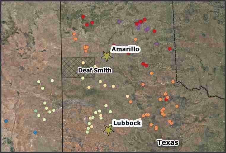
Spatial distribution of the data, graduated according to the depth of the groundwater.
Step 2: Exploratory data analysis
To delve deeper into data exploration, utilizing visual aids like histograms, box plots, scatter plots, and more can be incredibly helpful. In fact, these tools help to identify the distribution of your data and identify any outliers or errors that could adversely impact the accuracy of your results.
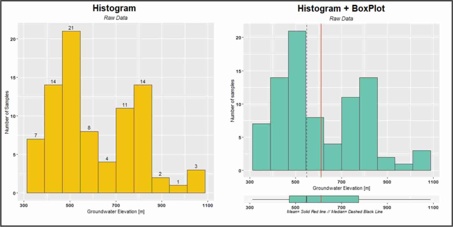
Left: histogram with the number of samples above each bin. Right: Histogram and boxplot together, with the mean and median.
Spatial analysis can become significantly more complex when data trends are present. These trends may result from topographic gradients, hydraulic gradients, variations in the source’s intensity, among other factors. Therefore, it is essential to detect and comprehend these trends before executing Universal Kriging. Notably, Universal Kriging determines trends based on coordinates, while external drift kriging employs other variables to define the trend.
There are situations in which Universal Kriging can directly address the trend of the data. However, more complex situations may require advanced techniques, like Regression Kriging, to model the trend and residual values separately.
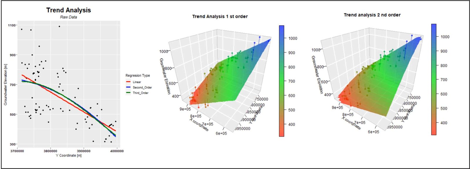
Left: The trend analysis is related to the Y coordinates. Center: A 3D model is displayed, showing the trend plane with a first-order polynomial and the values of the samples. Right: A 3D model is shown, displaying the plane of the trend with a second-order polynomial and the values of the samples.
Step 3: Data transformation
In some instances, it might be necessary to apply data transformation techniques before using Universal Kriging. This is especially relevant when dealing with data sets that have non-normal distributions. You can use different types of transformation, such as logarithmic, square root, or Box-Cox transformation, among others, to improve the data distribution. However, it is important to keep in mind that when applying Universal Kriging, the interpolation is performed on the residuals, not on the original data. Hence, it is crucial to ensure that the residual data have a normal distribution, or at least close to it, to guarantee precise results. Therefore, transforming the original data can be beneficial in enhancing the distribution of the residuals, leading to improved accuracy in the Universal Kriging outcomes.
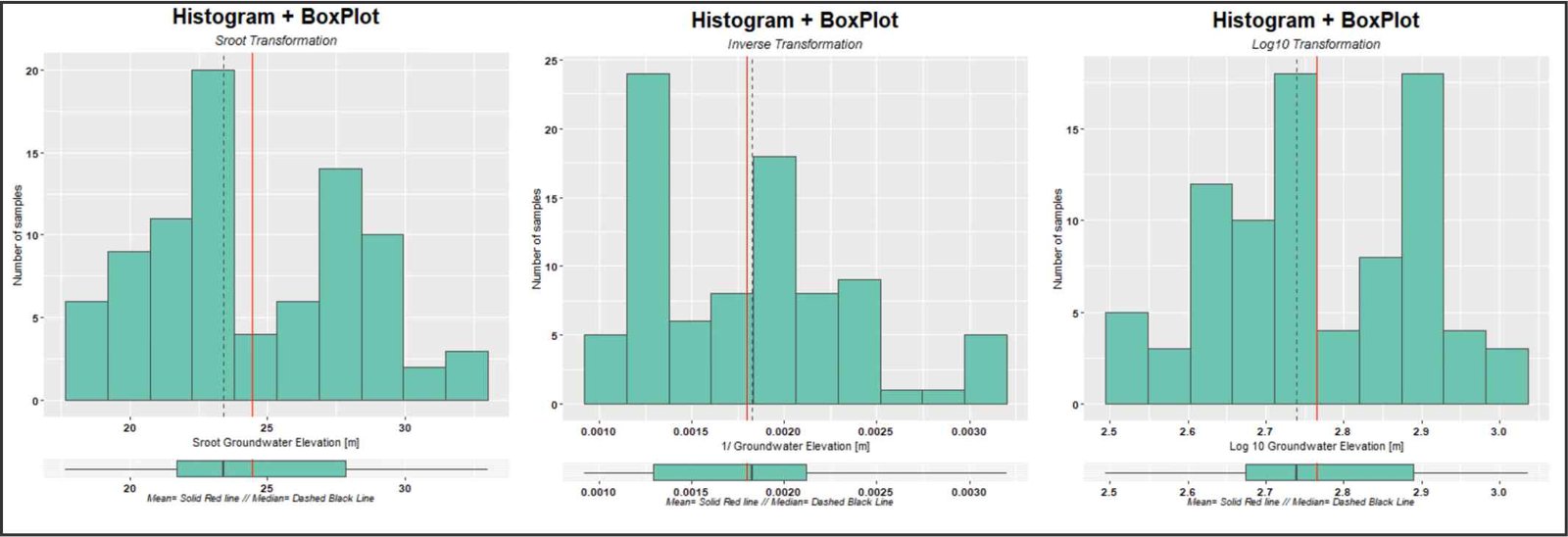
Transformation of the original data. Left: transformation based on the square root. Center: transformation based on the inverse. Right: transformation based on the base 10 logarithm.
Step 4: Exploratory data analysis on residual values.
To begin with, it is essential to mention that the variography analysis should be performed on the residual data, given that they will be utilized in the stochastic model during the Universal Kriging procedure. Moreover, the residual data has to satisfy specific criteria to be applicable for interpolation with Ordinary Kriging. In particular, it is imperative to conduct a data examination of the residual values to ensure their practicability.

Analysis of residual values. Left: histogram and box plot. Center: scatter plot of predicted and residual values. Right: bubble plot.
Step 5: Variographic Analysis.
After completing the exploratory analysis of the residual values, the next step is the variographic analysis. This analysis involves creating a mathematical model that explains the relationship between data variability and distance. The variogram is the function used to analyze this relationship. It describes how the data variance changes as the distance between them increases. Therefore, variographic analysis is an important step in determining the spatial correlation structure of the data, which is essential in the Universal Kriging process.
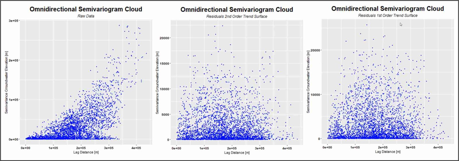
Omnidirectional variogram cloud. Variographic analysis. Left: original data, where the trend in the data is obvious. Center: data from residuals associated with the second-order trend surface. Right: data from residuals associated with the first-order trend surface.
To start, it’s worth mentioning that variographic analysis is an essential tool for comprehending the structure of spatial data. It allows obtaining different parameters, such as range, spatial autocorrelation, nugget effect, and partial sill. Besides, these parameters play a vital role in modeling and predicting spatial values as they help to understand the data’s variability and spatial relationship. For instance, the nugget effect signifies the unexplained variability of the variogram’s spatial structure, while the partial sill denotes the amount of variability that the spatial structure can explain. Furthermore, a high partial sill implies the data’s clear spatial structure, making it easier to model the variogram and conduct Universal Kriging.
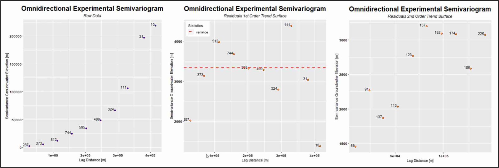
Variographic analysis of the omnidirectional experimental variogram. Left: original data, where the trend in the data is obvious and of quadratic nature. Center: data from the residuals associated with the first-order trend surface. Right: data from the residuals associated with the second-order trend surface.
Step 6: Selection of the variogram model
Once the variogram has been created, the next step is to select the model that best fits the data. The variogram model is a mathematical function that describes the spatial correlation structure of the data, which is quantified by the values of the range, the partial sill, and the nugget effect.
The selection of the proper variogram model is crucial to obtaining accurate results in Universal Kriging. However, there are several variogram models available, each with its own advantages and disadvantages. Some of the more common variogram models include the spherical model, the exponential model, and the Gaussian model.
Choosing the right variogram model is not an easy task and requires careful analysis based on the distribution of the variogram data and the selection of a suitable model. Therefore, it is recommended to try several variogram models to determine the most appropriate for the available data.
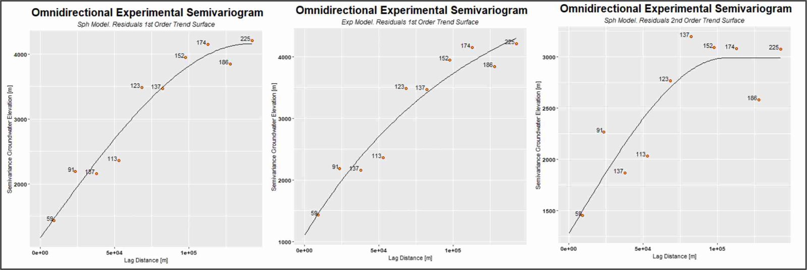
Left: spherical model fitted to residual values from the first-order trend surface. Center: exponential model fitted to residual values from the first-order trend surface. Right: spherical model fitted to residual values from the second-order trend surface.
Step 7: Validation and verification of the semivariogram model in Universal Kriging
After selecting the semivariogram model, it is crucial to validate and verify the model’s accuracy. One common way to do this is through cross-validation, where the data set is divided into groups, and the analysis is performed on each group to evaluate the model’s precision. It’s also important to use other evaluation mechanisms, such as comparing observed and predicted values.
Moreover, attention should be paid to the effect of neighborhood size and sampling density on the semivariogram model. Low sampling density can affect the model’s accuracy, while a too-large neighborhood can make the model too generalized and unable to capture the data’s local variability.
In summary, performing rigorous validation and verification of the semivariogram model in Universal Kriging is crucial to ensure accurate and reliable results.
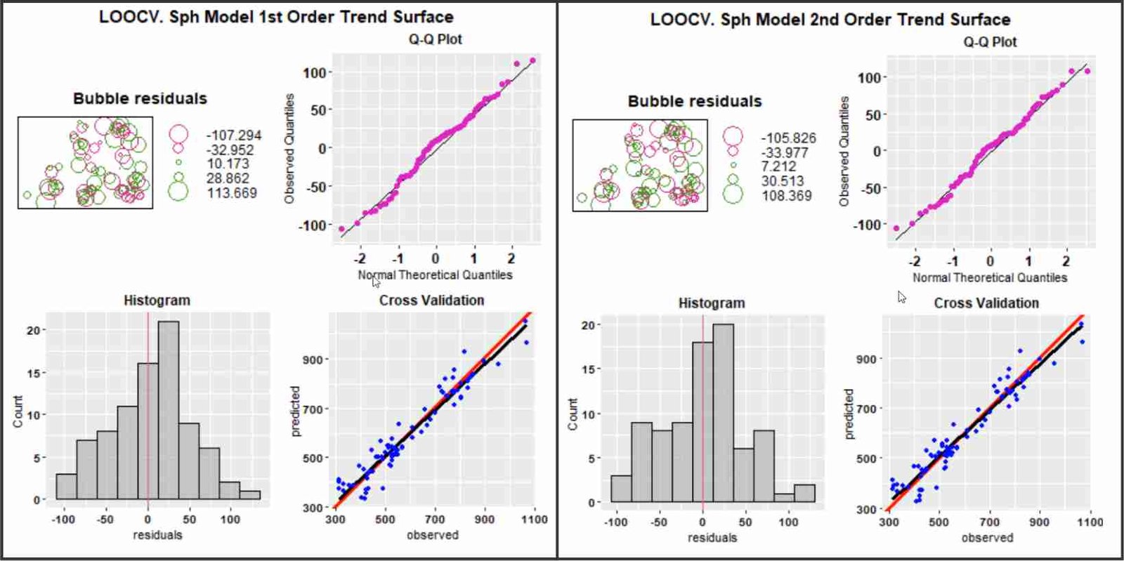
Leave-One-Out Cross-Validation (LOOCV) for the spherical model validation. On the left: kriging model based on residual values from the first-order trend surface. On the right: kriging model based on residual values from the second-order trend surface.
Step 8: Interpolation using Universal Kriging
Ultimately, Universal Kriging combines the stochastic (Ordinary Kriging) and deterministic (trend surface) models to produce a continuous surface. This integration occurs automatically based on information gathered in previous steps, including trend surface selection and semivariogram modeling. The resulting interpolation can then be utilized to generate contour maps and spatial distribution surfaces of data, which can aid in decision-making for environmental projects and related fields.
However, it’s important to remember that the accuracy of the interpolation heavily relies on the quality of the data used and the appropriate choice of semivariogram model. Both of these factors need to be carefully considered to achieve an accurate interpolation. Additionally, conducting cross-validation and other evaluation mechanisms is crucial in ensuring the reliability of the results.

Final result of interpolation.Left: the prediction map is displayed. Center: the variance or error map is shown. Right: a contour map is displayed, based on the values predicted.
Practical Example with QGIS and R, based on Universal Kriging
Next, we present the first tutorial in an eight-part video series featuring a practical exercise on Universal Kriging interpolation. The tutorial provides a detailed description of the eight main steps involved in the interpolation process. The project focuses on assessing the direction of groundwater flow for the establishment of residual nuclear waste sites in the United States.
Throughout the tutorial, the instructor takes the viewer through the various stages of the interpolation process, from data input and exploration to the application of the Universal Kriging method and the interpretation of the results. The creators designed the video to be easy to follow and accessible, allowing anyone with basic knowledge of GIS and R to participate in the exercise.
By the end of the eight-part video series, viewers will have gained practical experience in using Universal Kriging and will have acquired the skills to apply this method in their own projects. Various fields, including environmental science, geology, and other related fields that require the analysis of spatial data, can apply this knowledge.
Second Lesson of the Fourth Course on Geostatistics: Kriging/Cokriging Interpolation and Mapping, taught at https://giscourse.online/
Become an Expert in Geostatistics Today
If you’re looking to expand your skills in geostatistical analysis, this course is for you! The Fourth Geoestatistics Course on Interpolation and Kriging/Cokriging Mapping will provide you with a deep understanding of the different types of Kriging, as well as the ability to apply them to spatial data and present the results in maps in a completely professional way. With real examples and practical exercises using R integrated in QGIS, this course is the perfect choice for those who want to take their geostatistical analysis to the next level. Don’t wait any longer, access it now and start learning today!
Advantages of Universal Kriging
- Considers spatial data distribution, making it possible to estimate unknown values in areas without data.
- Universal kriging’s statistical approach produces accurate and reliable estimates of unknown values in the study area. This ensures greater confidence in the results obtained.
- Considers the spatial variability of data, resulting in more accurate estimates in areas with high variability. By doing so, the method can provide more precise information for decision-making purposes.
- Offers greater flexibility in trend selection due to the ability to include a deterministic trend in the data. This allows for more precise modeling of spatial data variability.
- Enables the estimation of uncertainty associated with interpolating unknown values. By providing this estimate, the method allows for a more accurate assessment of the accuracy of the results obtained.
Disadvantages of Universal Kriging
- The incorporation of a deterministic trend model in universal kriging can increase its complexity. As a result, it may require more time and effort to properly implement and analyze the results.
- Universal kriging may require more data to accurately model the trend, making it less accessible for smaller data sets. This can limit its usefulness in certain contexts.
- Universal kriging may suffer from decreased accuracy due to errors in the trend model specification. Proper understanding of trend structure is crucial for optimal results.
- Universal kriging is computationally demanding because it involves fitting both the trend and variability of the data. This can slow down the process and make it less efficient compared to other interpolation methods.
The 5 Most Important Questions Related to Universal Kriging
- What is universal kriging and how does it work?
Answer: Universal kriging is a spatial interpolation method that combines a deterministic model (trend) with a stochastic model (ordinary kriging). We use the stochastic model to model the spatial variability of the data, while we use the deterministic model to model any spatial trend in the data in universal kriging.
- What are the advantages of universal kriging over other spatial interpolation methods?
Answer: Universal kriging has a major advantage in its ability to handle spatially non-stationary data with trends. It is also a robust technique based on solid mathematical models, providing accurate and reliable results.
- How can I validate the results of universal kriging interpolation?
Answer: Cross-validation is a commonly used technique to evaluate the accuracy of universal kriging interpolation results. Other validation methods, such as comparison with independent validation data, can also be used.
- What are the advantages of universal kriging compared to other interpolation methods?
Answer: The universal kriging considers the variability and trend in spatial data for greater interpolation accuracy. It is used to predict values at any location within the study area, even where no samples have been taken.
- How is the trend model selected in universal kriging?
Answer: In universal kriging, the trend model is selected through exploratory data analysis. Additionally, this model can only be linear, which represents one of the major limitations of universal kriging. If a nonlinear model is desired, regression kriging needs to be used. The aim is to find a model that captures the spatial trend of the data without overfitting.
The 5 Most Common Questions Related to Universal Kriging
- What is universal kriging and how does it differ from ordinary kriging?
Answer: Universal kriging combines a deterministic trend model with a stochastic model. Unlike ordinary kriging, which is only a stochastic model. Ultimately, universal kriging allows for the incorporation of a spatial trend in the data.
- How is the semivariogram model selected in universal kriging?
Answer: The selection of the semivariogram model in universal kriging is based on variographic analysis of the data. Semivariogram models are fitted to the data to find the best fit of the variability.
- What are residual values in universal kriging?
Answer: Residual values are the difference between observed values and values predicted by the trend model. Universal kriging uses these residual values for spatial interpolation by utilizing the stochastic model of the semivariogram function.
- What are the advantages of universal kriging?
Answer: Universal kriging allows for the incorporation of a spatial trend and provides accurate estimates of unknown values. Additionally, it has the ability to provide uncertainty estimates, which is an important advantage in decision making.
- What are the limitations of universal kriging?
Answer: Universal kriging has limitations in the selection of the semivariogram model. This is due to the need to have sufficient and representative data to estimate trend and variability. Additionally, it is necessary for the data to meet assumptions of stationarity and normality for the stochastic model resolution.
#QGIS, #RStats, #Kriging, #SIG, #AnálisisEspacial, #VisualizaciónDeDatos, #Geoestadística, #CienciaDeDatos, #CódigoAbierto, #Teledetección.
