Ordinary Kriging 5-Step Practical Guide.
Welcome to the fascinating world of Ordinary Kriging! Did you know that this spatial interpolation technique is widely used across various fields, from weather prediction to air quality assessment and pollution distribution? Then, if you’re interested in learning more about how to apply this powerful tool in your spatial analysis, you’re in the right place. In this ultimate guide, created by the GeoRGB Community and available at https://giscourse.online, we present to you the 5 key steps to successfully perform Ordinary Kriging. By carefully following these steps, you’ll be well on your way to obtaining precise and reliable results in your scientific projects. Moreover, you’ll discover how this technique will help you better understand spatial data and make informed decisions in your research. So, join us on this exciting journey, and let’s learn together!
Step 1: Collecting Data for Working with Ordinary Kriging
Data collection is a critical step in the Ordinary Kriging process, as the accuracy and reliability of the interpolation results depend on the quality and representativeness of the data. In this regard, it is crucial to clearly define the purpose of the data collection and the study area. This step will allow you to identify what types of data are needed and what data sources are available.
For data collection, different sources can be used, such as weather stations, remote sensors, and field measurements. These data can include measurements of air quality, precipitation, temperature, pollution, and other environmental parameters. It is important to ensure that the data is representative of the study area and covers a sufficient period of time to capture the temporal and spatial variations of the environmental parameters.
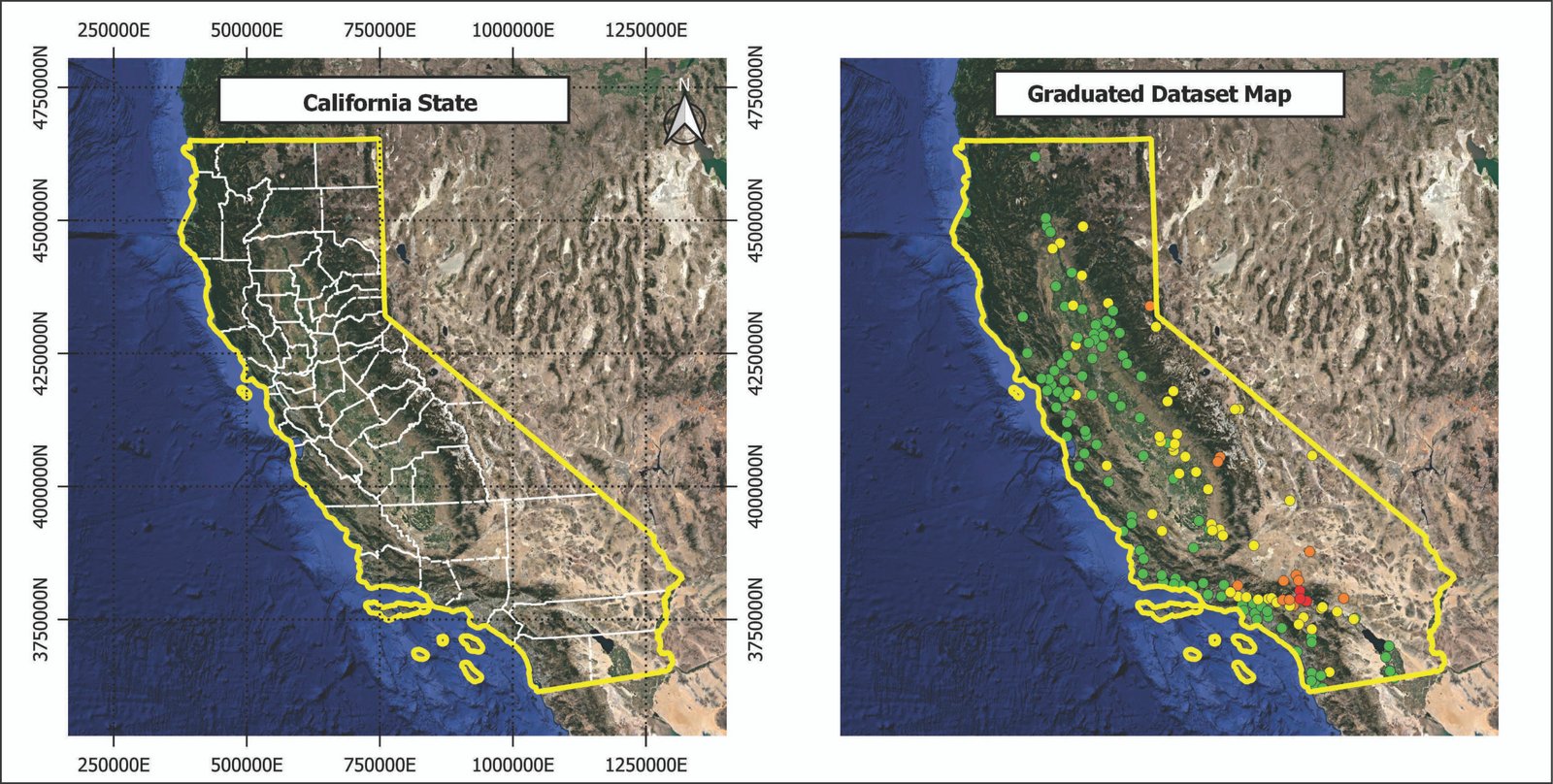
Left: Map showing the state of California. Right: Map showing the spatial distribution of the data.
After the data has been collected, it is important to conduct quality control to ensure the accuracy and reliability of the data. Various techniques, such as calculating summary statistics and detecting outliers and errors, can be used to achieve this. Additionally, it is crucial to adequately document the data and collection methodology to ensure transparency and reproducibility of the results. Through proper documentation of the data and methodology, one can guarantee the credibility and reliability of the findings.
Step 2: Exploratory Data Analysis for Ordinary Kriging
In this step, a basic statistical analysis of the data is conducted to identify the existence of outliers, the distribution of variables, and the presence of correlations.
During the exploratory data analysis, various techniques can be used, such as visualization and descriptive statistics. Visualization is a useful tool to understand the spatial and temporal distribution of the data, and maps and charts can be utilized to identify patterns and trends. On the other hand, descriptive statistics are used to summarize and analyze the data, which may include calculating measures of central tendency and dispersion, as well as identifying possible outliers. Both techniques are crucial for identifying any issues that may affect the Ordinary Kriging analysis and for determining the best approach to handle such issues.
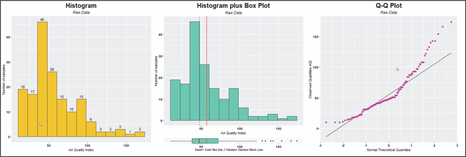
Left: Histogram with an asymmetric distribution. Center: Same histogram, but with the addition of a box plot. Right: Q-Q plot indicating the lack of normality of the data.
In addition, the exploratory data analysis should consider the stationarity of the process. In fact, stationarity implies that the distribution of the data is constant in time and space, which is important for the use of kriging. If the process is non-stationary, transformation techniques can be used to obtain a stationary distribution. Therefore, it is crucial to identify whether the data is stationary or not during the exploratory data analysis to ensure accurate and reliable results for the Ordinary Kriging analysis.
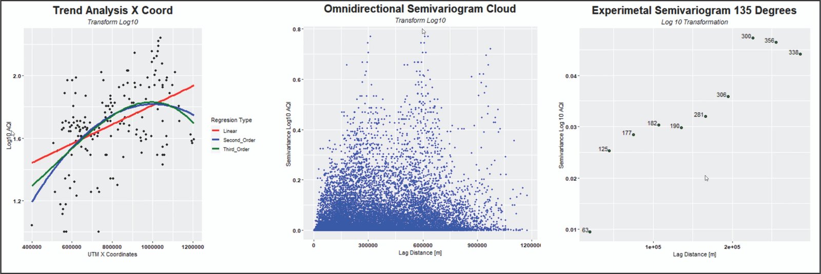
Left: Trend analysis in relation to X coordinates. Center: Cloud of omnidirectional semivariogram. Right: Experimental semivariogram with a direction of 135 degrees.
Step 3: Model selection in Ordinary Kriging
In the process of selecting a model for ordinary kriging, the choice of the variogram model is particularly important. For instance, the most commonly used variogram models are the spherical, exponential, and Gaussian models. In particular, the spherical model is appropriate for data with short spatial correlation, while the exponential model is used for data with moderate spatial correlation. Finally, the Gaussian model is used for data with long spatial correlation.
It is important to note that the choice of variogram model can significantly affect the interpolation results, so the model that best fits the data and the application purpose should be carefully selected. In addition, it is important to appropriately adjust the parameters of the variogram model, which may involve different model adjustments and evaluations.
Overall, the selection of the variogram model is a crucial part of the ordinary kriging process. The appropriate variogram model will depend on the nature and spatial distribution of the data. It is also important to consider the application purpose and the temporal and spatial scale of the problem. Careful selection of the variogram model and proper parameter adjustments are crucial for achieving precise and reliable interpolation.
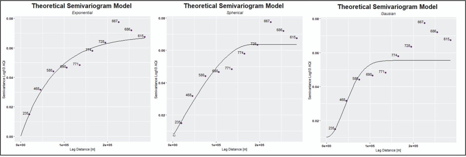
Left: Exponential model. Center: Spherical model. Right: Gaussian model.
Step 4: Ordinary Kriging Interpolation
The next step is to perform interpolation using the selected variogram model. This involves creating a continuous surface from the sample data. It is important to note that the interpolation results depend on the sampling density of the data. The higher the sampling density, the more accurate the interpolation results will be.
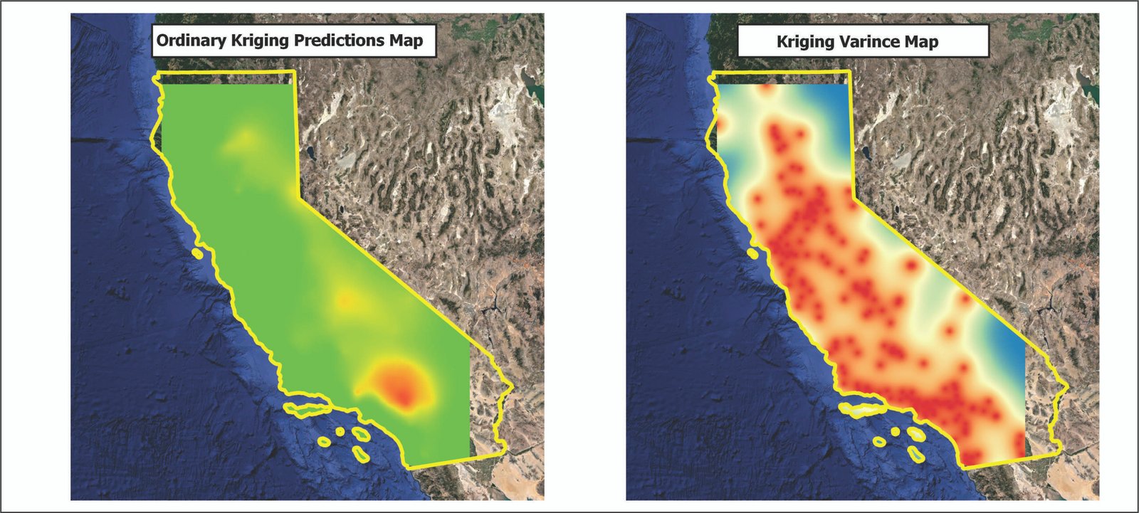
Left: Map showing the prediction according to the Kriging model. Right: Map showing the variance according to the Kriging model.
In this step, the Kriging model is applied to interpolate the values of the variable of interest at locations where no data is available. It is important to keep in mind that the accuracy of the results will depend on the size and distribution of the sample data, as well as the selected variogram model. It is also important to note that the interpolation will not provide accurate information in areas that are beyond the scope of the sample data. Therefore, caution should be exercised when interpreting the interpolated values in areas where no sample data is available.
Step 5: Validation and Verification of the Ordinary Kriging Model
In validation, different techniques can be used. One of the most popular techniques is cross-validation, which is used to evaluate the accuracy of the interpolation model. Cross-validation involves partitioning the sample data into a training set and a validation set. The training set is used to create the Kriging model, and the validation set is used to evaluate the accuracy of the model. Cross-validation can provide information on the model’s ability to predict unknown values and the accuracy of the predictions in different areas of the spatial field.
On the other hand, verification is used to evaluate the quality of the interpolation results. This may involve comparing the interpolation results with the sample data and with other reference data, such as independent measurements or estimates from other interpolation techniques. Verification is an important way to ensure that the interpolation results are accurate and reliable, and to detect possible errors or biases in the Kriging model.

Leave-One-Out Cross-Validation (LOOCV) for the Spherical Model. Left: Bubble map for the residual values. Center: Histogram of the residuals. Right: Scatter plot showing the relationship between observed and predicted values.
In summary, validation and verification are critical steps in the ordinary Kriging process. These steps allow us to evaluate the accuracy and reliability of the interpolation results, and to detect possible errors or biases in the model. It is important to use appropriate validation and verification techniques. With these techniques, we can ensure the accuracy and reliability of the interpolation results. Additionally, we can make informed decisions based on the interpolated data.
Practical Example with QGIS and R based on Ordinary Kriging
Below, we present the first tutorial in a series of 8 videos that demonstrate a practical exercise in ordinary Kriging. The tutorial includes a detailed description of the five main steps involved in performing interpolation using ordinary Kriging. The project focuses on the evaluation of air pollution in the state of California, in the United States.
First Lesson of the fourth Geoestatistics Course: Kriging/Cokriging Interpolation and Mapping, taught at https://giscourse.online/
Become an Expert in Geostatistics Today
If you’re looking to expand your skills in geostatistical analysis, this course is for you! The Fourth Geoestatistics Course on Interpolation and Kriging/Cokriging Mapping will provide you with a deep understanding of the different types of Kriging, as well as the ability to apply them to spatial data and present the results in maps in a completely professional way. With real examples and practical exercises using R integrated in QGIS, this course is the perfect choice for those who want to take their geostatistical analysis to the next level. Don’t wait any longer, access it now and start learning today!

Advantages of Ordinary Kriging
- Precision: Ordinary Kriging provides accurate results when estimating unknown values at locations where no measured data is available.
- Flexibility: Ordinary Kriging can be applied in a variety of contexts and with different types of data.
- Interpretability: Ordinary Kriging provides an easy-to-interpret mathematical model that greatly facilitates the understanding of the spatial relationships between the data.
- Efficiency: Ordinary Kriging is computationally efficient and allows for handling large datasets quickly and effectively.
- Updatability: The ordinary Kriging model can be easily updated with new data to improve the results of the interpolation. This leads to a more accurate estimation in areas where new data has been collected.
Disadvantages of Ordinary Kriging
- Data quality dependence: The accuracy of ordinary Kriging depends on the quality of the input data. Therefore, contexts with low data quality can pose a real challenge.
- Sensitivity to parameter choices: The choice of model parameters in ordinary Kriging can significantly affect the accuracy of the results, which can be difficult to determine in contexts with unknown spatial variability.
- Inability to handle non-stationary data: In ordinary Kriging, the choice of parameters can significantly affect the accuracy of the results. Therefore, it is difficult to determine them in contexts with unknown spatial variability.
- Not suitable for large study areas: Ordinary Kriging can be computationally intensive and may not always be suitable for large study areas, which can limit its applicability in some contexts.
- Incomplete spatial uncertainty: Ordinary Kriging provides point estimates of unknown values where no measured data is available, but it does not provide a complete spatial uncertainty, which can be a limitation in contexts where spatial uncertainty is important.
The 5 Most Important Questions Related to Ordinary Kriging
- How can ordinary Kriging be applied to different types of data?
The ordinary Kriging technique can be applied to different types of data, such as point, areal, and volumetric data. This technique estimates unknown values on a grid of points using a spatial correlation function.
- How can the model parameters be selected to maximize the accuracy of the ordinary Kriging results?
Parameters such as the variogram model and neighborhood size can be selected by fitting the variogram function and validating the model using techniques such as cross-validation.
- What are the limitations of ordinary Kriging in terms of spatial variability and data input quality?
Ordinary Kriging is affected by spatial variability and the quality of the input data, such as the presence of outliers and lack of samples in specific areas.
- How can uncertainty be incorporated into ordinary Kriging results?
Uncertainty can be incorporated into the results by generating uncertainty maps based on the variogram function and cross-validation of the model. Additionally, uncertainty can be quantified by estimating the standard error.
- What are the alternatives to ordinary Kriging, and how do they compare in terms of accuracy and efficiency in different contexts?
Alternatives include inverse distance weighting, spline, Delaunay triangulation, and neural network-based methods, and the choice will depend on the context and properties of the data.
The 5 Most Common Questions Related to Ordinary Kriging
- What is the function of variogram and how is it used in ordinary kriging?
The variogram function is a mathematical function that describes the spatial variability of data. In ordinary kriging, it is used to model spatial correlation and adjust model parameters.
- What is the impact of input data quality on the accuracy of ordinary kriging?
The quality of input data can significantly affect the accuracy of ordinary kriging. The presence of outliers and lack of samples in specific areas can affect the accuracy of results. Therefore, some cases may require the application of data preprocessing techniques and selection of representative samples.
- How can ordinary kriging be implemented in GIS software?
Many GIS software, such as ArcGIS and QGIS, have tools that allow users to implement ordinary kriging. The user can input the data, select the model parameters, and generate maps of results and uncertainty.
- How can spatial anisotropy be handled in ordinary kriging?
Spatial anisotropy varies in different directions, and to handle it, anisotropic kriging can be applied. This technique models spatial correlation in different directions and adjusts model parameters accordingly.
- How can non-normality in data be addressed in ordinary kriging?
Non-normality in data can affect the accuracy of ordinary kriging. However, data transformation techniques can be used to address non-normality. There are different techniques for transforming data, such as logarithmic and square root transformations, among others.
#QGIS, #RStats, #Kriging, #GIS, #SpatialAnalysis, #DataVisualization, #Geostatistics, #DataScience, #OpenSource, #RemoteSensing
