Kriging External Drift: the most powerful guide.
Welcome to the fascinating world of Kriging with External Drift, a crucial methodology in spatial interpolation. A wide range of scientific fields, not limited to mineralogy, hydrogeology, geology, and climatology, extensively employ this technique, highlighting its significance within the Earth sciences. If you harbor an interest in acquiring an in-depth understanding of the application of this robust method in your geospatial analyses, you’ve aligned with an apt resource.
Presented to you by the GeoRGB Community, this authoritative guide, accessible at https://giscourse.online, lays out the crucial steps to successfully execute Kriging with External Drift. Adhering closely to these guidelines, you’ll pave the way towards delivering precise and trustworthy outcomes in your environmental endeavours.
Moreover, this technique will enhance your comprehension of spatial data, empowering you to make well-informed decisions in your investigations. Don’t delay, embark on this enlightening journey with us and elevate your learning experience!
What is kriging with External Drift?
Kriging with External Drift (KED) is a method employed in spatial interpolation. This approach comes into play when we have a secondary variable, also known as an external variable, which exhibits a correlation with the primary variable under study. We leverage this correlation to enhance the precision of our estimations.
At the heart of Kriging with External Drift is a key concept: the primary variable can be envisioned as a blend of a deterministic function, often referred to as the “drift,” and a stochastic or random element. The secondary variable steps in to shape the drift. Hence, the primary variable Z at any given spatial location “s” can be articulated as a sum of a deterministic function μ(s) and a random term ε(s).
Z(s)= μ(s)+ε(s)
Picture this, you are on a mission to forecast the pollutant concentration in a river, which is your primary variable. You’ve discovered that there’s a correlation between this concentration and the water temperature, your external variable. This is where Kriging with External Drift comes into play. By applying this technique, you can notably sharpen the accuracy of your predictions.
Kriging with External Drift really shines when you have readings of the secondary variable across the entire interpolation grid, but only a few samples of the primary variable in the study area. In these scenarios, Kriging with External Drift steps up to the plate, offering more precise estimates than your standard ordinary kriging.
Kriging with External Drift bears a similarity to Universal Kriging, but there’s a key divergence between the two. While Universal Kriging relies on geographical coordinates to identify trends in data, Kriging with External Drift pivots to an external variable to lay out these trends.
Data preparation for Kriging with External Drift
Step 1: Data Collection
Gathering data stands as the initial step towards any geospatial analysis, and here are a few key pointers to keep in mind during this stage:
a. Pinpointing Samples: You require data from locations where samples or readings have been procured. Geographical coordinates or a projected coordinate system, often UTM, are generally utilized for this purpose. This information is vital for the spatial analysis and the operation of Kriging with external drift.
b. Primary Variable: You will need details about the variable that you plan to interpolate. This could be measurements of diverse types like mineral concentrations, precipitation values, the depth of groundwater, and so on.
c. Drift Variables (External): These represent additional variables that you anticipate could unravel the variations in your key variable. We usually harvest external variables from remote sensor data sources, including but not limited to satellite imagery, LiDAR, radars, and Digital Elevation Models (DEMs). Alternatively, we can calculate these variables in a conventional office setting, based on features discernible in terrain images, topographical maps, morphological maps, among others. Such resources facilitate the computation of relevant distances such as proximity to coastlines or rivers, and more.
It’s crucial to grasp that the external variable needs to be available at every pixel of the interpolation grid and precisely at the sample or measurement site. This condition is key to ensuring the proper functioning of the interpolation method. Further into this tutorial, we will explore how to handle the interpolation grid.
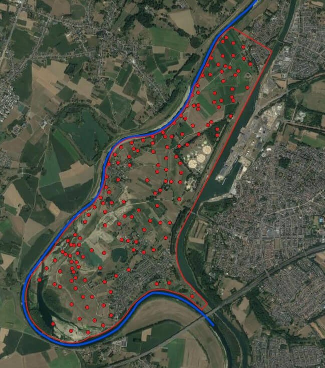
Spatial distribution of data related to the zinc concentration within the defined study area. The River Meuse borders this area.
Step 2: Data verification
Ensuring the accuracy of your data is a cornerstone step in any analysis, safeguarding the reliability and validity of your results. Here are a few important points to take note of:
a. Consistency Assurance: A thorough check of your data to rule out any inconsistent or out of place values is necessary. For example, when dealing with temperature data, a reading of 273 degrees Celsius would raise a red flag in most cases.
b. Unit Harmony: It is vital to ensure all your measurements are harmonized in the same units. If you are handling distance data and find measurements in both kilometers and miles, it is time to convert all the data to a common unit for easy and effective comparison.
c. Mapping Locations and Measurements: Make sure that the measurements align perfectly with their respective locations. If you are working with a temperature measurement dataset and a geographical location dataset, each temperature value must be correctly paired with its geographical counterpart.
d. Duplicate Scrutiny: Replicated data can throw your results off track. So, it iss worth scanning for duplicate observations in your dataset and strategizing how best to manage them.
e. Outlier Evaluation: Outliers, the values in your data that distinctly stand out due to errors or authentic observations, can notably sway your results.
Always remember, data verification is not a one off process, it is an ongoing endeavor that should run parallel to your entire analysis.
Step 3: Exploratory data analysis (EDA)
When dealing with KED, exploratory data analysis forms a key part of the process, giving you a deeper understanding of your data’s structure and characteristics:
a. Spatial Visualization: Given that you are dealing with geospatial data, it is crucial to visualize your data spatially. This could involve mapping out scatter plots to display the location of your sampling points and how the values of your target variable and the external variable are spread across the area. These spatial insights can help you spot patterns or zones of interest.
b. Distribution Analysis: It is beneficial to get a sense of your target variable and the external variable’s distribution. You might want to construct histograms and/or boxplots and conduct normality tests for this purpose. These steps can help you get a better understanding of the data’s spread and identify any potential skewness or outliers.
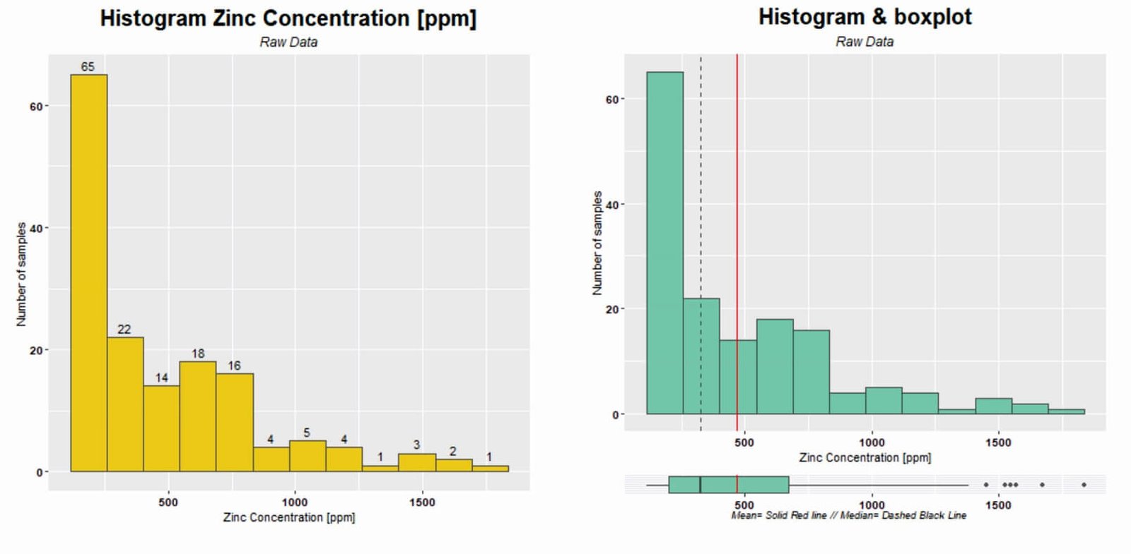
Left: A histogram with the number of samples displayed above each bin. Right: A combined histogram and box-and-whisker plot, showcasing the mean and median.
c. Data Transformation and Normality: It is a common assumption in many statistical and geostatistical methods, such as KED, that data adheres to a normal distribution. However, reality often breaks away from this ideal. To pursue normality in KED, you have got to investigate the normality of your data first. Histograms, Q-Q plots, boxplots, or specific statistical tests can accomplish this.
If your data decides to defy normality, you will have to step in with transformations. This could be logarithmic, square root, or perhaps the Box-Cox transformation. After reshaping the data, take a moment to check back on its normality. When you are ready, employ your transformed data in the KED process. However, do not forget that to make sense of the final result or maps, you might need to backtrack and undo the transformation you applied earlier.
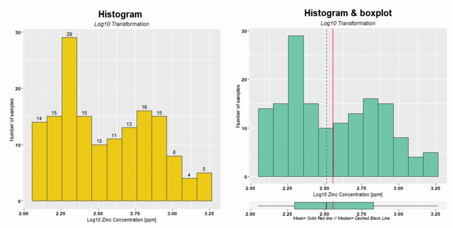
Left: Histogram of the transformed data, with the number of samples specified above each bin. Right: Combined histogram and box plot for the transformed data, displaying the mean and median.
d. Trend Analysis: KED operates under the assumption that there is a drift function influencing the variation in the primary variable. As such, it is crucial to perform a trend analysis to unearth any hidden patterns in your data, which might involve creating trend graphs. Furthermore, since an external variable is used to help explain part of the variation in the primary variable, it is vital to understand the interplay between the two.
For this purpose, you can create scatter plots and perform correlation analysis, while regression analysis can be saved for a detailed exploration of the drift function. The fact that the primary and external variables are located in the same place significantly simplifies this type of analysis.
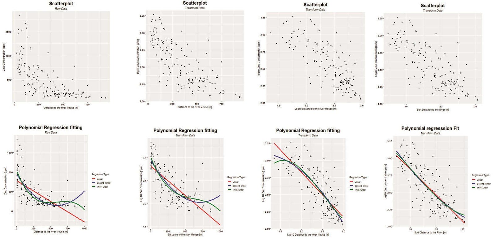
Scatter plots are displayed at the top. These graphs depict the relationship between the primary and the external variables, incorporating both transformed and original data sets. Further down, we present scatter plots adapted to fit polynomial trend models. The intention here is to pinpoint the model that adheres most closely to the data, a determination based on their specific transformations.
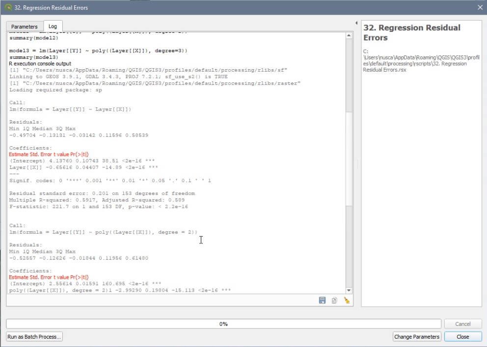
Regression analysis executed with the QGIS interface.
e. Variogram Analysis: Variographic analysis serves as a vital instrument for deciphering the structure of spatial data. Through this method, various parameters can be obtained, including range, nugget effect, and partial sill. These elements are significant for modeling and predicting spatial values, as they allow for an understanding of data variability and its spatial relationship.
For instance, the nugget effect represents the variability not accounted for by the variogram’s spatial structure, while the partial sill indicates the amount of variability that can be explained through spatial structure. If the partial sill is high, it signifies a clear spatial structure in the data, which aids in variogram modeling and carrying out KED.
After constructing the variogram, the next step involves selecting the model that best fits the data. The variogram model is a mathematical function describing the spatial correlation structure of the data. This structure is perfectly quantified with the values of the range, partial sill, and the nugget effect.
Choosing the appropriate variogram model is critical for accurate results in kriging with external drift. There are various variogram models available, each with their own merits and shortcomings. Some of the more common variogram models include the spherical model, the exponential model, and the Gaussian model.
Selecting the variogram model is no small task. This decision is based on the distribution of the variogram data and the selection of a suitable model. Therefore, it is necessary to conduct a careful analysis in order to make a sound selection of the variogram model. In the end, it is advisable to test several variogram models to determine the most suitable one for the available data.

Analysis of the variogram and adjustment of the spherical model, implementation with RStudio.
Step 4: Creating the interpolation grid
The interpolation grid constitutes a network of points sprawled across the geographic landscape. Here, I will detail the fundamental steps for its construction:
a. Define the geographic extent: The initial stride towards developing an interpolation grid involves outlining the geographic boundaries of your study area. This demarcated extent must encompass all the locations you aim to estimate.
b. Determining the Grid Resolution: The grid resolution pertains to the size of each individual cell or pixel within the grid. The smaller the cell size, the greater the resolution of your grid, thereby refining your interpolation. However, it is crucial to note that a finer resolution demands increased computational time and storage space. Typically, the grid resolution is dictated by the minimum distance between samples of the primary variable. Nevertheless, in this instance, it could also be conditioned by the pixel dimensions of the raster pertaining to the external variable.
c. Constructing the Grid: Once you have established the extent and resolution, you can proceed to build the grid. This involves generating a matrix of points that blanket your entire geographic extent at the specified resolution.
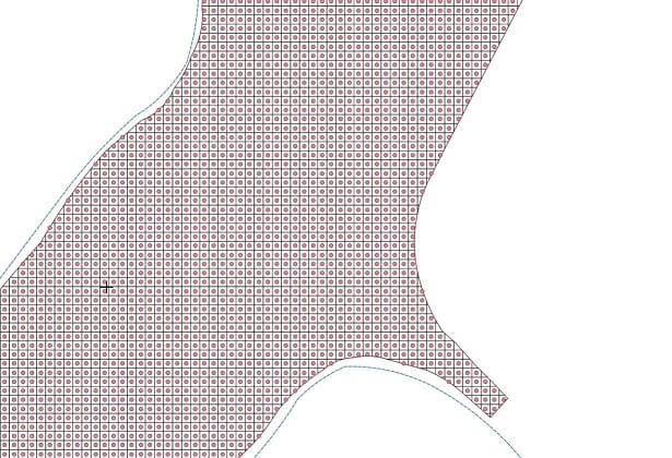
Data matrix associated to the interpolation grid.
d. Allocating External Variable Values to the Grid: This is an integral and critical element of KED, which truly distinguishes it from any other kind of interpolation grid. Your task is to assign a value from your external variable to each point in your interpolation grid. You can accomplish this by utilizing data obtained from remote sensors, DEM, topographic maps, or other geospatial data resources.
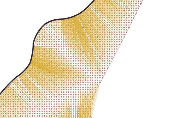
Calculation of the external variable in the data matrix. In this case, the external variable is the minimum distance to the river.
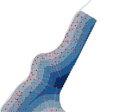
We visualize the distance to the river through a final raster and represent it with red dots from the original dataset.
Step 5: Interpolation using Kriging with External Drift
Ultimately, Kriging with External Drift constitutes the synthesis of a stochastic and a deterministic model. The KED method cohesively merges these two models, a capability afforded by information procured in previous steps, such as the selection of the external drift and the semivariogram model. We can use the resulting interpolation to create contour maps and surfaces representing spatial data distribution. Such data could be instrumental for decision-making processes in environmental projects, and other related disciplines.
The precision of the interpolation is strongly contingent upon the quality of the data used. Furthermore, the choice of the external drift and semivariogram model is critical. It is thus essential to thoughtfully consider both these elements in order to achieve an accurate interpolation. Cross-validation must be employed to ensure the trustworthiness of the outcomes. Furthermore, it is important to explore the application of other evaluative mechanisms to strengthen the overall reliability and robustness of the results.
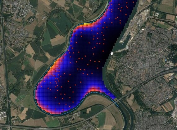
Final result of the interpolation.
Step 6: Cross validation for kriging with external drift
Statisticians often use cross-validation to evaluate a model’s generalizability. In the context of Kriging with External Drift, we can use this technique to validate the interpolation’s accuracy and robustness.
Here, I present a basic scheme for implementing K-Fold cross-validation in KED. However, it is relevant to mention other techniques. A popular example is Leave-One-Out Cross-Validation (LOOCV):
- We divide the dataset into subsets, typically using 5 or 10 subsets. These subsets should be representative of the original dataset.
- For each subset, fit the KED model using the remaining data. That is, all data except those of the current subset.
- Utilize the fitted model to predict values in the current subset. We didn’t use these data in fitting the model.
- Compare the predictions with actual values and record some measure of error (for instance, mean squared error).
- Repeat steps 2-4 for each subset.
- Calculate an average of the recorded error measures. This will provide an estimate of how well the KED model will perform with new data.
Remember that, generally, it is desirable to have an adequate number of samples to carry out solid validation. If the sample size is exceedingly small, the uncertainty in the estimation might be high. In such a case, it’s crucial to consider other sources of information. Auxiliary data or insights from an expert in the area can enhance the quality of predictions.
Practical example with QGIS and R, based on Kriging with External Drift.
We are excited to present an engaging, two-part tutorial that unfolds a hands-on exercise on KED. This tutorial will guide you through the intricate process of interpolation, step by step. The focus will be on estimating zinc concentration for the identification of contaminated soils.
Through this tutorial, the mentor will walk you through each phase of the interpolation process. It covers everything from data entry and exploration to the application of KED. The tutorial culminates with a detailed interpretation of the results, allowing you to glean the maximum value from each stage of the exercise.
We have designed this tutorial to be intuitive and accessible. Indeed, it caters to individuals with foundational knowledge of GIS and R. Clear explanations and visual illustrations facilitate an understanding of all concepts.
Upon completion of this tutorial, you will have gained valuable hands-on experience in using Kriging with External Drift. Moreover, you’ll be equipped with the necessary skills to apply this method in your own projects. You can apply the knowledge acquired here across a variety of fields, such as geology and environmental sciences.
Our ultimate goal is for you to acquire solid competencies in spatial data analysis, utilizing a variety of tools. In this way, you will be able to confront real-world challenges and make significant contributions in your field of study or work. You are just a click away from embarking on this exciting journey into the world of Kriging with External Drift!
Fourth lesson of the fourth Geostatistics course: Kriging/Cokriging interpolation and mapping, taught at https://giscourse.online/
Become an expert in geostatistics today!
If you are on a mission to enhance your geostatistical analysis skills, look no further! This Geostatistics Course on Kriging/Cokriging Interpolation and Mapping will immerse you in the diverse world of Kriging types, thereby streamlining your spatial data analysis and professional map creation. With real-world examples and hands-on exercises using R integrated into QGIS, this course undeniably stands as the prime choice for those aspiring to elevate their geostatistical analysis prowess. Do not hesitate, seize this opportunity now and kickstart your learning journey today!

5 Advantages of kriging with External Drift
Kriging with External Drift (KED) stands as a robust and adaptable geostatistical method for the interpolation of spatial data. Below, I showcase five key advantages of employing KED:
a. Integration of Additional Information: Unlike ordinary Kriging, KED allows for the integration of additional information in the form of an external variable. This can help enhance the accuracy of interpolation, particularly when the external variable is strongly correlated with the variable of interest.
b. Management of Spatial Trends: KED can proficiently manage spatial trends in data, which proves especially useful in scenarios where data exhibit systematic change in a specific direction. The model incorporates the drift function to achieve this.
c. Estimation of Uncertainty: Much like other Kriging methods, KED provides not only an estimation of values at unsampled locations, but also a measure of the uncertainty associated with these estimations. This can be invaluable for risk-based decision making.
d. Optimized Interpolation: KED, akin to other Kriging methods, utilizes optimal estimation theory. This implies that, under certain assumptions, KED estimates are statistically the best possible.
e. Flexibility: KED is flexible in terms of the form of the drift function that can be used. This can be a linear function of spatial coordinates, a function of external variables, or a combination of both. This allows for the adaptation of the model to the specific structure of your data.
5 Disadvantages of kriging with External Drift:
Kriging with External Drift carries many advantages. However, it is essential to consider its limitations when employing this method. Here, we list five of them:
a. Statistical Assumptions: KED, like other Kriging methods, makes certain assumptions about the data, including stationarity and normality. If our data do not meet these assumptions, we risk obtaining biased or inaccurate KED estimates.
b. Selection of the External Variable: Choosing the external variable in KED can be challenging. If the external variable does not correlate well with the variable of interest, its inclusion might not enhance, and could even degrade, the precision of the interpolation.
c. Computational Complexity: KED can be computationally intensive, particularly for large data sets and high-resolution interpolation grids. This can make KED less practical for real-time applications or for very large datasets.
d. Need for an Interpolation Grid: KED requires the creation of an interpolation grid with values of the external variable for each grid point. This can be a challenge if data for the external variable is not available across the full extent of the grid.
e. Difficulty of Interpretation: Although KED can provide more accurate estimates than other interpolation methods, interpreting the results can be more challenging. This is due to the inclusion of the external variable and the complexity of the KED model itself.
Despite its drawbacks, KED is valuable for interpolating spatial data. Its effectiveness relies on its appropriate usage and understanding of its limitations.
The Top 5 Most Frequently Asked Questions About Kriging with External Drift:
What is “external drift” in KED? The “external drift” refers to the inclusion of an external variable in the Kriging model.We use this external variable, which can be any measurable feature expected to correlate with the variable of interest, to explain part of the spatial variation in the data.
How do I choose the external variable in KED? The choice of the external variable should be based on your understanding of the system you are studying. Ideally, the selected variable should have a strong correlation with the variable of interest and should be available at all locations for which we want to make estimates.
Why do I need to check the normality of my data in KED? It is essential to verify normality in KED because this method assumes that the residuals (differences between the observed and the estimated trend values) follow a normal distribution. If your data does not comply with this assumption, you may find your estimates to be biased or inaccurate. In such a case, you should consider transforming your data to ensure normality before applying KED.
How do I handle trends in my data when using KED? The drift function in KED enables the handling of trends in the data. By incorporating a drift function into your model, you can effectively model the systematic variation in your data that cannot be explained solely by spatial autocorrelation.
When should I use KED instead of ordinary Kriging? KED can be useful when you have an external variable that is strongly correlated with your variable of interest, or when your data show a spatial trend that cannot be adequately managed by ordinary Kriging.
#QGIS, #RStats, #Kriging, #GIS, #SpatialAnalysis, #DataVisualization, #Geostatistics, #DataScience, #OpenSource, #RemoteSensing.
