CoKriging Complete Guide: Save Money in Environmental Projects
Quick Summary
Cokriging: Revolutionary Geostatistical Method for Multi-Variable Analysis
Cokriging
Co-kriging (also written as CoKriging or cokriging) is an advanced geostatistical method used in spatial analysis that enhances the traditional kriging technique by incorporating multiple correlated variables. This approach allows for more accurate predictions of spatial phenomena by leveraging the relationships between different data sets, leading to richer and more precise spatial models. Cokriging is particularly effective in complex environments where analyzing multiple variables simultaneously provides a more comprehensive understanding of the spatial relationships.
Step 1: Collecting Data for Working with Ordinary Cokriging
1.1) Introduction to data collection
1.2) Primary and secondary variables
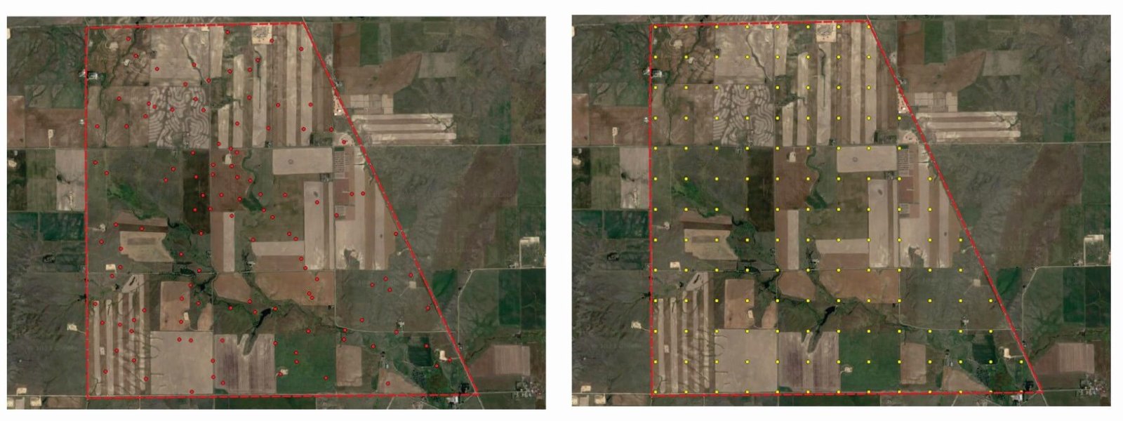
Cokriging Sampling
Left: Map displaying the spatial distribution of soil chloride concentration plus soil electrical conductivity. Right: Map illustrating the sampling locations for only soil electrical conductivity across the site.
Step 2: Exploratory Data Analysis for Ordinary CoKriging
In the second step of our ordinary co-kriging process, we engage in Exploratory Data Analysis (EDA). This critical phase involves an in-depth examination of our dataset to identify underlying patterns and characteristics that will inform our subsequent analyses. EDA is far more than a preliminary review; it is an integral, thorough investigation that forms the foundation for accurate and effective modeling.
2.1) Data Distribution
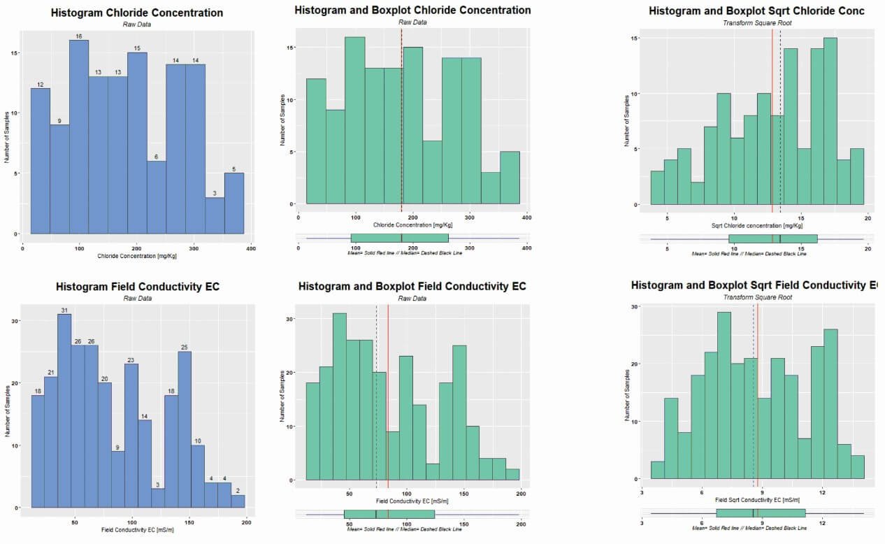
In this stage of ordinary cokriging, we concentrate on analyzing the data distribution using histograms and boxplots. These tools are crucial for understanding the distribution patterns of both primary and secondary variables.
Histograms provide an initial look into the dataset, showcasing the distribution of data points across various intervals. This visual representation aids in identifying central tendencies, dispersion, and any deviations from normal distribution, such as skewness.
Boxplots further this analysis by offering insights into the variability and range of the data. They are particularly useful for identifying outliers and understanding the quartile distribution, both of which are essential for ensuring the robustness and reliability of our cokriging analysis.
Our analysis often reveals the need to transform both primary and secondary datasets to achieve a stronger correlation. This decision, based on the EDA findings, aims to improve the effectiveness of the ordinary co-kriging process. By aligning the distribution and correlation of both variables, we lay the groundwork for more precise and insightful spatial analysis in subsequent steps.
Cokriging histogram analysis
Left: Histograms showing chloride concentration (top) and electrical conductivity (bottom), each bin displaying the number of samples. Both histograms exhibit distributions close to normality. Center: The same histograms, now enhanced with box plots that better illustrate central tendency measures and the absence of outliers. Right: The same histograms post a square root transformation, showcasing how the data distribution has been modified.
2.2) Data Correlation
Proceeding to the next critical phase in ordinary cokriging, we focus on analyzing the interrelationships between our variables. This phase is pivotal, as it involves a detailed examination of how these variables interact, going beyond mere statistical correlations to understand their true connections.
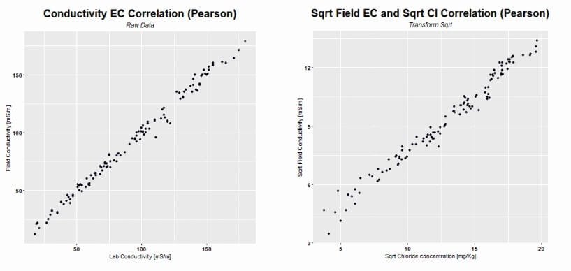
First, we assess the correlation between field-measured and laboratory-measured electrical conductivity. A strong correlation here is essential. A weak or non-existent correlation signals potential issues in data collection or instrument calibration, while a high correlation, ideally near 1, confirms the reliability of our field data. A moderate correlation may indicate the need for recalibration of field instruments using laboratory results for increased accuracy.
Next, we examine the correlation between soil chloride concentration and field-measured electrical conductivity. It’s crucial to establish that this correlation is not only statistically significant but also meaningful. We aim to verify that the observed electrical conductivity changes are due to chloride concentration, not other factors, to avoid misleading correlations.
We use scatter plots to evaluate these correlations: one comparing field and laboratory electrical conductivity, and another comparing field electrical conductivity with soil chloride concentration. A linear correlation close to 1 in these plots is a positive indicator for proceeding with co-kriging. Conversely, a weak correlation suggests that cokriging may not be suitable, and ordinary kriging might be a better alternative.
In summary, this Data Correlation phase is a thorough validation step, ensuring the relationships between our variables are valid and robust, thereby laying a strong foundation for the accurate implementation of the ordinary cokriging model.
CoKriging Correlation Analysis
The image illustrates scatter plot analyses: on the left, it reveals the correlation between electrical conductivity measurements taken in the field and those obtained in the laboratory; on the right, it highlights the relationship between field electrical conductivity and soil chloride concentration.
2.3) Data Trend Analysis
CoKriging Trend Analysis
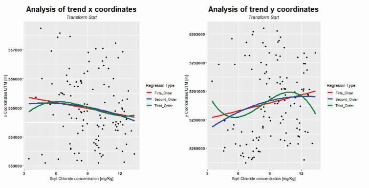
The image features two scatter plots for data trend analysis. On the left, it displays a plot of the X coordinates against the square root of the chloride concentration, while the right plot shows the Y coordinates against the same. Both plots include regression lines of first, second, and third order. However, none of these regression lines clearly indicate any distinct trend in the data.
Step 3: Model selection in Ordinary CoKriging
In Step 3 of ordinary cokriging, we address the critical task of model selection, which involves a detailed variographic analysis. This process is akin to that in ordinary kriging for analyzing primary and secondary variables, but co-kriging introduces an additional complexity with the use of cross-semivariograms. This element adds depth to our analysis, differentiating it from kriging.
In cokriging, unlike kriging which focuses on semivariograms of individual variables, we intertwine these analyses through cross-semivariograms. This integral step examines the interactions between variables, moving beyond mere preference to a necessity. This analysis directs us to adopt the regionalized model of coregionalization, known for its stringent requirements. This model is essential to accurately capture the spatial correlations between our variables in co-kriging.
Selecting the appropriate model is both challenging and imperative. It ensures that our cokriging model is not only statistically sound but also finely tailored to the unique characteristics and interrelations of our dataset. This careful selection process is crucial for refined and accurate spatial analysis, enabling us to maximize the potential of ordinary co-kriging for insightful spatial predictions.
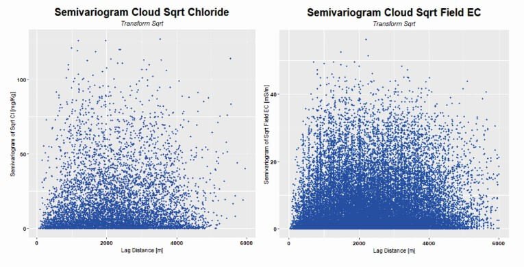
3.1) Semivariogram Cloud
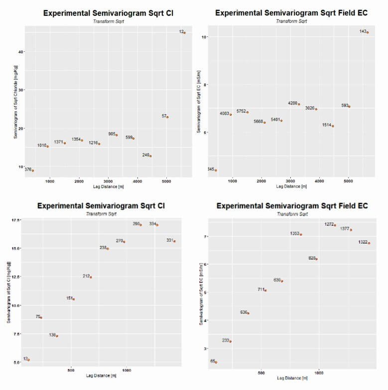
3.2) Experimental Semivariogram
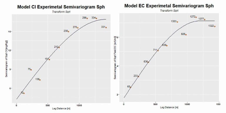
3.3) Model selection
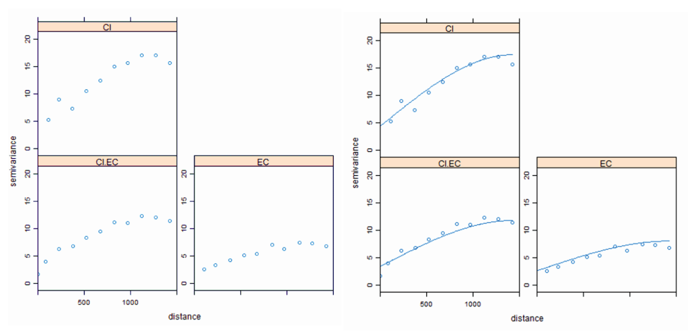
In this step, we concentrate on the quantitative aspects of our CoKriging analysis, focusing on critical parameters such as the nugget effect, sill, and range. This phase is essential as it determines the specific model for our analysis, tailored to the unique characteristics of our data.
A crucial part of this process involves quantifying the nugget effect, representing small-scale variation or measurement error, and the sill, the threshold beyond which variables stop correlating with increasing distance. We also determine the range, the distance up to which the spatial variables are correlated. A unique requirement of the Linear Model of Coregionalization, used in our CoKriging analysis, is that both primary and secondary variables must have the same range and model type, although their nugget effects and sills may vary. This requirement can be challenging as it restricts the applicability of CoKriging in some cases.
When fitting models to the semivariogram, we can proceed manually or automatically, selecting the model that best fits the data while ensuring consistency in model and range for both variables. This may require compromises to meet the criteria of the Linear Model of Coregionalization.
We won’t go into the details of model fitting here, as it was covered in our previous discussion on Ordinary Kriging. The methods for achieving a good fit are similar, and further guidance is available in our course on structural analysis. Our goal is to select a model that adheres to CoKriging’s requirements and accurately represents our spatial data.
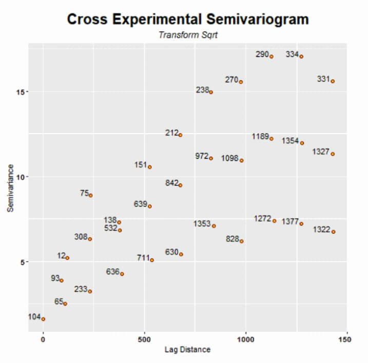
3.4) Linear Model of Coregionalization
We now focus on the Linear Model of Coregionalization, a key element in our ordinary co-kriging approach. This sophisticated statistical model is crucial for capturing the complex interdependencies and combined variability of our primary and secondary variables. The careful alignment of cross-semivariograms with each variable’s individual semivariogram, a task undertaken in earlier phases, is pivotal here. This alignment greatly influences the model’s effectiveness in spatial interpolation and prediction.
A major advantage at this stage is the use of R, a potent tool that facilitates the simultaneous adjustment of all three semivariograms – those of the primary and secondary variables, and their cross-semivariogram. This automatic adjustment in R is vital to meet the strict criteria of the Linear Model of Coregionalization, streamlining the process and ensuring compliance with the required standards for a more reliable spatial analysis.
Using R in implementing the Linear Model of Coregionalization allows us to integrate and fine-tune parameters like range, sill, and nugget effect. This method not only combines datasets but also unravels the intricate relationships between different spatial phenomena. It leads to a deeper understanding of the spatial dynamics within our study area, which is indispensable for revealing the nuanced interactions between variables and achieving more accurate spatial predictions.
Step 4: Interpolation Grid for Kriging/CoKriging
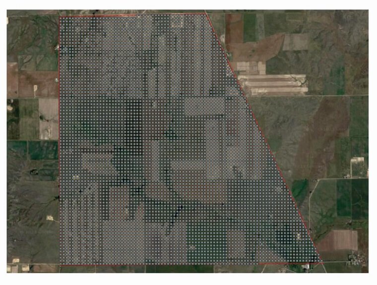
In this step of ordinary cokriging, we emphasize the significance of choosing an optimal grid size and shape for interpolation. This choice crucially affects both the accuracy of the spatial predictions and the computational efficiency. The selection process considers several factors: the spatial distribution and variance of data points, the scale of the study area, and the nature of spatial relationships among the variables.
Selecting an appropriate grid involves a careful balance. A too-large grid may miss important spatial details, while a too-small grid can lead to excessive computation without meaningful increase in accuracy. This configuration is not arbitrary but a strategic decision. It ensures that cokriging fully utilizes the available data, thereby maximizing the reliability and precision of the predictions.
Cokriging Interpolation Grid
The map shows the interpolation grid based on dimensions of 60 x 60 meters.
Step 5: Ordinary Kriging Interpolation
In this phase, our focus turns to ordinary kriging interpolation, following our comprehensive analysis of chloride concentration through co-kriging. Armed with a deep understanding of the variable, we can now effectively implement ordinary kriging. This method serves as a comparative tool, allowing us to evaluate its results against those obtained from ordinary cokriging.
The groundwork established in earlier steps becomes advantageous here. With a thorough grasp of the distribution and spatial structure of chloride concentration, implementing ordinary kriging is streamlined. We can utilize previously established insights and parameters, like the variogram model and its range, making this phase more efficient.
Ordinary kriging is not just a procedural step; it significantly enriches our understanding of the spatial behavior of the variable across the study area. By comparing the outputs of ordinary kriging with those of co-kriging, we gain valuable insights into each method’s capacity to model spatial data. This comparative analysis illuminates the nuances in how each technique manages spatial dependencies and variability, assisting us in selecting the most suitable method for our spatial analysis objectives.
In essence, this step not only contributes to our repository of results but also deepens our comprehension of spatial data modeling. It provides a critical perspective on the strengths and limitations of each geostatistical approach, guiding our decision-making in spatial analysis.
Ordinary Kriging
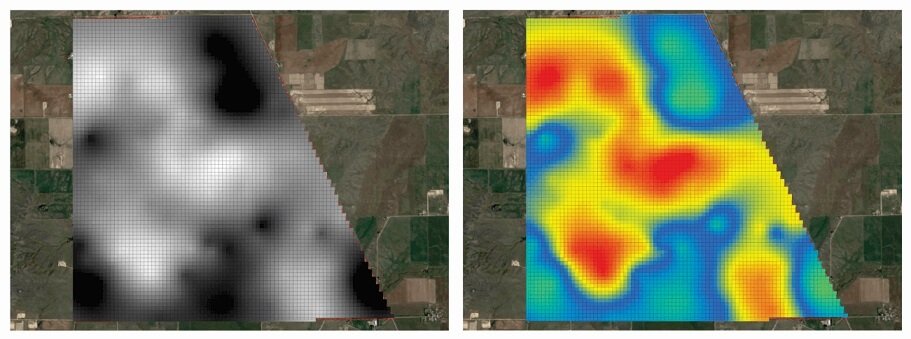
The left map displays the interpolation of the square root of chloride concentration using ordinary kriging, while the right map shows the same interpolation, but with values reverted back to their original scale, effectively undoing the data transformation.
Step 6: Ordinary CoKriging Interpolation
In this step, we progress to the core aspect of our spatial analysis: ordinary cokriging interpolation. This method, an advancement in interpolation techniques, builds upon our preliminary work and integrates insights from both primary and secondary variables. Ordinary co-kriging is distinguished by its ability to factor in the spatial correlation between variables, thus enhancing the precision and dependability of our results.
At this juncture, we apply the models calibrated from our variographic analysis and the Linear Model of Coregionalization. Our focus is the primary variable, chloride concentration. However, ordinary cokriging goes beyond mere prediction at unsampled locations. It’s a comprehensive process that considers the joint variability and mutual influence of chloride concentration and electrical conductivity.
The effectiveness of ordinary co-kriging lies in its detailed approach to spatial prediction. It leverages the secondary variable, in this case, electrical conductivity, to provide context and augment information, resulting in more accurate estimations. As we implement this method, we closely observe how the inclusion of secondary data refines our understanding of spatial patterns and trends in the primary variable. This step is essential for achieving a deeper and more nuanced understanding of our spatial data.
Ordinary CoKriging
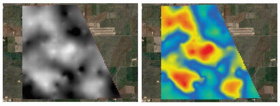
On the left, the map illustrates the interpolation results using ordinary cokriging for the square root-transformed chloride concentration data. The right map, in contrast, presents these interpolated results after converting the values back to their original chloride concentration scale, thereby reversing the initial square root transformation.
6.1) Comparison of Interpolation Results: Kriging vs CoKriging
In this section, we focus on analyzing the distinctions in spatial structures revealed by ordinary kriging and co-kriging. A noteworthy observation from this comparison is that the spatial structures identified in ordinary kriging appear to be larger compared to those detected in cokriging. This suggests that co-kriging, with its integration of secondary data, is able to refine the interpretation of chloride concentration, revealing smaller, more intricate spatial structures. This difference underscores the enhanced resolution that cokriging brings to our spatial analysis. It highlights how the incorporation of additional variables in co-kriging contributes to a more detailed and nuanced understanding of the spatial distribution of chloride concentration, as opposed to the broader patterns typically identified through ordinary kriging alone. This comparative analysis not only illustrates the strengths of each method but also sheds light on the complexity and diversity of spatial patterns in environmental data.
Step 7: Cross Validation Ordinary Kriging/CoKriging Models
In validation, different techniques can be used. One of the most popular techniques is the leave-one-out cross-validation (LOOCV), which is used to evaluate the accuracy of the interpolation model. Cross-validation involves partitioning the sample data into a training set and a validation set. The training set is used to create the kriging/cokriging model, and the validation set is used to evaluate the accuracy of the model. Cross-validation can provide information on the model’s ability to predict unknown values and the accuracy of the predictions in different areas of the spatial field.
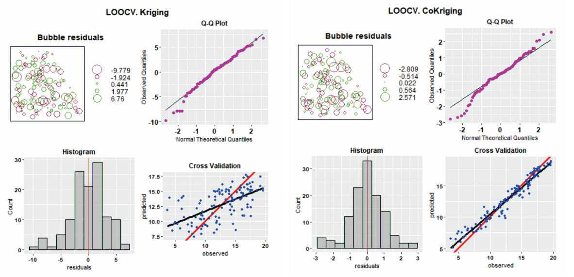
Kriging Vs CoKriging Cross Validation
In the image, we observe a comparison of the cross-validation results (LOOCV – Leave-One-Out Cross-Validation) for both kriging and co-kriging, showcased across four different types of graphs.
Practical Example with QGIS and R based on Ordinary CoKriging
Below, we introduce the first video tutorial showcasing a practical exercise in ordinary cokriging. This tutorial provides an in-depth walkthrough of the seven key steps required for conducting interpolation using ordinary co-kriging. Centered around the assessment of soil contamination by chloride, the tutorial offers a comprehensive guide, from initial data collection to the final interpolation analysis. Each step is elaborated with detailed explanations and insights, making it an invaluable resource for those looking to apply ordinary cokriging in environmental studies, particularly in the context of soil contamination evaluation.
Fifth Lesson of the fourth Geoestatistics Course: Kriging/Cokriging Interpolation and Mapping, taught at https://giscourse.online/
Become an Expert in Geostatistics Today
If you’re looking to expand your skills in geostatistical analysis, this course is for you! The Fourth Geoestatistics Course on Interpolation and Kriging/Cokriging Mapping will provide you with a deep understanding of the different types of kriging and co-kriging, as well as the ability to apply them to spatial data and present the results in maps in a completely professional way. With real examples and practical exercises using R integrated in QGIS, this course is the perfect choice for those who want to take their geostatistical analysis to the next level. Don’t wait any longer, access it now and start learning today!

Advantages of CoKriging
- Improved Accuracy: Cokriging utilizes both primary and secondary data sets, allowing for more precise interpolation. By incorporating additional relevant variables, it often achieves higher accuracy in predicting spatial distributions compared to methods that use a single variable.
- Efficient Use of Data: Co-kriging is particularly beneficial in scenarios where the primary variable of interest is difficult or expensive to sample extensively. The method leverages more easily obtainable secondary data, thus maximizing the utility of all available information.
- Reduction of Estimation Variance: By using two or more related variables, cokriging typically reduces the estimation variance compared to ordinary kriging. This means that the predictions are generally more reliable and closer to the true values.
- Flexibility in Application: Co-kriging is versatile and can be applied across various fields such as environmental science, mining, agriculture, and meteorology. Its ability to integrate different types of data makes it a powerful tool for a wide range of spatial analysis tasks.
- Cost Reduction in Interpolating Target Variable: Cokriging can significantly reduce the costs associated with data collection for the primary variable of interest. By effectively utilizing secondary data, which is often less expensive or more readily available, co-kriging reduces the need for extensive and costly sampling of the primary variable. This makes it a cost-efficient choice for spatial analysis, especially in scenarios where obtaining primary data is resource-intensive.
Disadvantages of CoKriging
- Complexity in Implementation: Co-kriging is a more complex method compared to ordinary kriging. It requires a thorough understanding of both primary and secondary data, including their relationships and statistical properties, making the process more intricate and challenging to implement correctly.
- Data Requirement Constraints: For cokriging to be effective, the secondary variable must be strongly correlated with the primary variable. Finding such a suitable secondary variable can sometimes be difficult, limiting the applicability of the method in certain scenarios.
- Increased Computational Demands: The inclusion of additional variables in co-kriging leads to higher computational demands. This can be a significant drawback, particularly when dealing with large datasets or limited computational resources.
- Modeling Challenges: Cokriging requires the construction of cross-semivariograms in addition to the semivariograms for each variable. This adds an extra layer of complexity in model fitting and can be challenging, especially in ensuring that the models for the primary and secondary variables are compatible.
- Risk of Misinterpretation: Due to its complexity, there’s a greater risk of misinterpreting the results or making errors in the co-kriging process. Incorrect model selection, inadequate understanding of the variables’ relationship, or errors in data processing can lead to inaccurate results.
The 5 Most Important Questions Related to CoKriging
1. What is the correlation between the primary and secondary variables?
The correlation between the primary and secondary variables in cokriging is essential. It should be strong and positive, indicating that changes in one variable are reliably reflected in the other. Co-kriging assumes that the secondary variable provides additional, relevant information about the spatial distribution of the primary variable. If this correlation is weak or non-existent, the effectiveness of cokriging is significantly diminished.
2. How do you select the appropriate secondary variable?
The selection of an appropriate secondary variable is a balance of correlation strength and practicality. The ideal secondary variable should have a strong spatial correlation with the primary variable and be easier or cheaper to sample. This could mean using variables that are more frequently observed, require less complex technology to measure, or are available from existing datasets.
3. What are the challenges in modeling and interpreting cross-semivariograms?
Modeling and interpreting cross-semivariograms involve understanding how two variables interact spatially at various distances. The challenges here include accurately estimating these interactions and ensuring the model fits well with empirical data. Misinterpretation or poor model fit can lead to inaccurate predictions. The complexity increases with the non-linearity of relationships and the presence of multiple scales of spatial variation.
4. In what scenarios is cokriging more advantageous than ordinary kriging?
Cokriging is particularly advantageous in scenarios where the primary variable is difficult, expensive, or time-consuming to sample extensively. Examples include environmental monitoring, mineral exploration, and meteorological forecasting. In such cases, a readily available secondary variable can significantly enhance the spatial prediction of the primary variable, making co-kriging a more efficient choice despite its additional complexity.
5. How does cokriging impact the accuracy and reliability of spatial predictions?
Co-kriging generally improves the accuracy and reliability of spatial predictions compared to ordinary kriging. By incorporating a secondary variable, it provides a more nuanced understanding of spatial variation. This can lead to more accurate predictions, especially in areas with limited primary data. The reliability of cokriging predictions hinges on the strength of the correlation between the primary and secondary variables and the appropriateness of the chosen semivariogram models.
The 5 Most Common Questions Related to Ordinary CoKriging
1. What is the difference between ordinary kriging and cokriging?
The primary difference lies in the use of data: ordinary kriging utilizes a single variable for interpolation, while co-kriging incorporates a secondary variable that is statistically correlated with the primary one. Cokriging leverages this additional variable to enhance the accuracy and reliability of the spatial predictions.
2. Can cokriging be used for all types of spatial data?
Co-kriging is versatile but not universally applicable. It’s most effective when the primary and secondary variables have a strong spatial correlation. Its suitability depends on the nature of the dataset, the relationship between variables, and the specific goals of the analysis.
3. What are the computational requirements for cokriging?
Cokriging, being more complex than ordinary kriging, typically requires more computational power. This is due to the need to manage and analyze larger datasets (primary plus secondary data) and the additional computations for cross-semivariograms and model fitting.
4. How do you validate the results obtained from cokriging?
Validation of cokriging results typically involves cross-validation techniques, such as Leave-One-Out Cross-Validation (LOOCV), to assess the model’s predictive performance. Metrics like the mean squared error (MSE) or the root mean squared error (RMSE) are used to evaluate the accuracy of the prediction.
5. What is the difference between cokriging and kriging with external drift (KED)?
While both co-kriging and kriging with external drift (KED) use additional variables, they differ in their approach. Cokriging simultaneously interpolates the primary variable and secondary variable, considering the spatial correlation between them. KED, on the other hand, uses the secondary variable as a ‘drift’ or trend in the interpolation of the primary variable, typically assuming a linear relationship between the primary variable and the external drift. KED is generally simpler and less computationally intensive than cokriging, but might not capture complex relationships as effectively as co-kriging.
About the Author: Marcel A. Cedrez
Marcel A. Cedrez (MarcelGeoRGB) is the founder and director of the GeoRGB Community at https://giscourse.online. He is a hydrogeologist and geospatial analyst with over a decade of experience in environmental projects. Marcel holds a Bachelor and Master’s degree in Geology from the University of Barcelona, a postgraduate diploma in Hydrogeology from the Polytechnic University of Catalonia, and a Master’s degree in GIS and Remote Sensing from the University of Girona.
Marcel is the creator of several QGIS and R applications for geostatistics and the developer of the “Sampling Time” plugin, which uses AI to optimize sampling strategies. He has produced over 140 video tutorials on his GeoRGB Community YouTube channel and teaches specialized courses in geostatistics, GIS, LiDAR, and hydrogeology. You can see his projects and open-source code on his GitHub profile.
Connect with Marcel:
- Linkedin: linkedin.com/in/marcel-cedrez
- YouTube: GeoRGB Community
- GitHub: MarcelGeoRGB
Keywords: #QGIS, #RStats, #Kriging, #CoKriging, #Cokriging, #Co-kriging, #GIS, #SpatialAnalysis, #DataVisualization, #Geostatistics, #DataScience, #OpenSource, #RemoteSensing, #EnvironmentalMonitoring, #ResourceEstimation
